Three ways to Understand the Mixed Product of Vectors! 向量混合积的三种理解

When it comes to \(a \cdot (b \times c)\), what’s in your head?

1 Hello!

This property of vector operation bother me for a loooooong time:

Mixed product¹: \[ \boxed{ a \cdot (b \times c) = b \cdot (c \times a) = c \cdot (a \times b). } \tag{1}\]

¹ Also known as “scalar triple product”.

This says nothing but the mixed product is unchanged under a circular shift.

You will understand it in this article!

2 Three Approaches to the Mixed Product

Lemma

Lemma 1 Let \(a, b, c \in \mathbb{R}^3\), then \[ a \cdot (b \times c) = \begin{vmatrix} | & | & | \\ a & b & c \\ | & | & | \end{vmatrix} \]

Once this is established, we can use the fact that: \[ \begin{vmatrix} | & | & | \\ a & b & c \\ | & | & | \end{vmatrix} = \begin{vmatrix} | & | & | \\ b & c & a \\ | & | & | \end{vmatrix} = \begin{vmatrix} | & | & | \\ c & a & b \\ | & | & | \end{vmatrix} \] to prove Equation 1.

Now let’s understand Lemma 1 in three different ways!

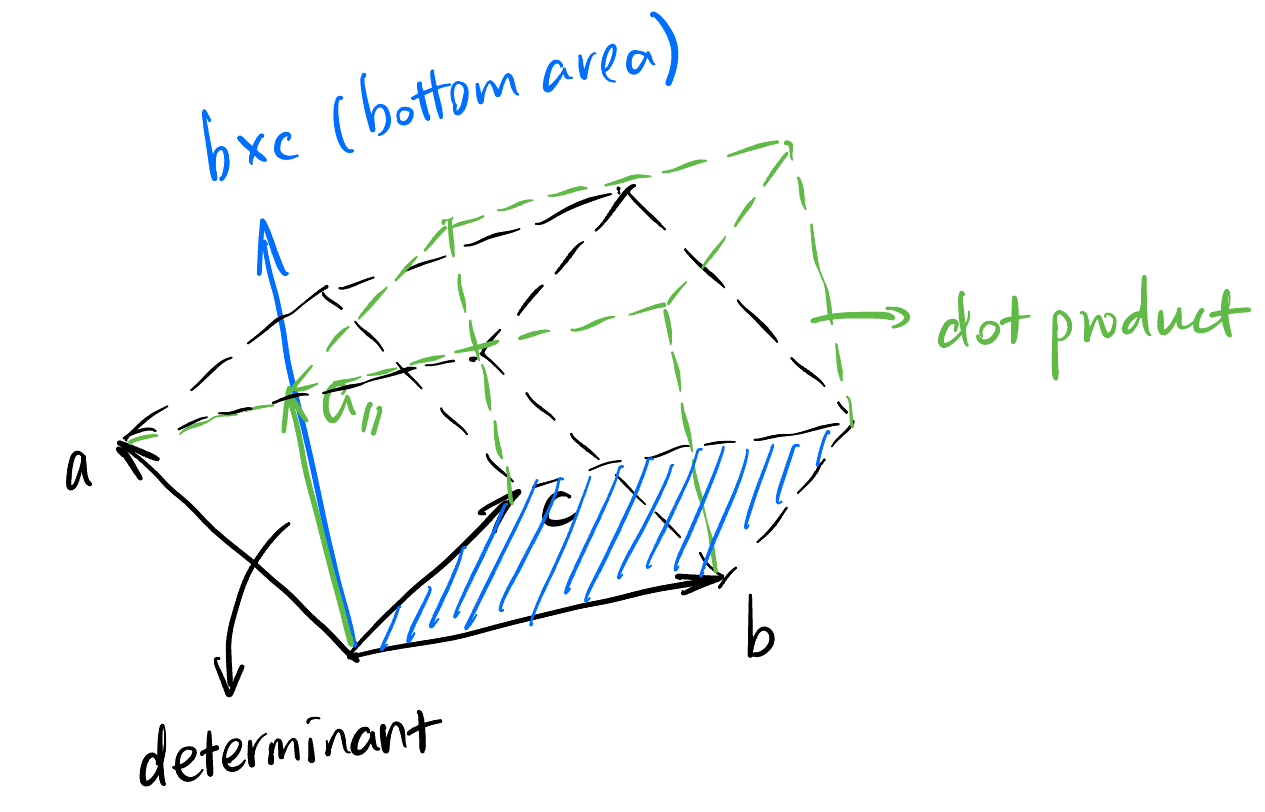
2.1 Geometric Approach

See Figure 1, dot product make the slanted black box straight but maintains its volume.

Figure 1: Geometric proof of Lemma 1

2.2 3b1b Approach

I called this “3b1b Approach” because this method is inspired by a great mathematician Grant Sanderson. “3b1b” is the name of his Youtube channel.

In a video created by him, there is a very interesting function \(f: \mathbb{R}^3 \to \mathbb{R}\): \[ f(x) = \begin{vmatrix} | & | & | \\ x & v & w \\ | & | & | \end{vmatrix} \tag{2}\] which takes in a vector in \(\mathbb{R}^3\) and output a number in \(\mathbb{R}\) (\(v\) and \(w\) are predefined and fixed).² Now I claim that:

² Functions from a vector space to a scalar is often referred to as a functional.

Claim

Theorem 1 The functional \(f\) in Equation 2 is linear, i.e., \[ f(x + y) = f(x) + f(y), \forall x, y \in \mathbb{R}^3 \] and \[ f(\alpha x) = \alpha f(x), \forall \alpha \in \mathbb{R}. \]

This is trivial.

There is another theorem³:

³ There is a video created by myself that explains this in detail.

Riesz Representation Theorem (reduced version)

Theorem 2 Every linear functional in \(\mathbb{R}^n\) induces a vector \(p \in \mathbb{R}^n\) such that \[ f(x) = x \cdot p, \forall x \in \mathbb{R}^n. \]

Therefore, Equation 2 becomes \[ \boxed{ x \cdot p = \begin{vmatrix} | & | & | \\ x & v & w \\ | & | & | \end{vmatrix} } \tag{3}\]

Mnemonic device inspired by Equation 3

The Equation 3 gives us a way to write the cross product in a more “dot-product” way: \[ v \times w = \begin{vmatrix} \hat{\imath} & v_1 & w_1 \\ \hat{\jmath} & v_2 & w_2 \\ \hat{k} & v_3 & w_3 \end{vmatrix} \] because the result \(v \times w = (v_2w_3 - v_3w_2)\hat{\imath} + (v_3w_1 - v_1w_3)\hat{\jmath} + (v_1w_2 - v_2w_1)\hat{k}\) is very much like a dot product! Remember \(v_2w_3 - v_3w_2, v_3w_1 - v_1w_3, v_1w_2 - v_2w_1\) are just three numbers unless you you associate each number with a direction.

If you feel uncomfortable with this notation, there is more: \[ \operatorname{curl} F \equiv \nabla \times F = \begin{vmatrix} \hat{\imath} & \frac{\partial}{\partial x} & F_x \\ \hat{\jmath} & \frac{\partial}{\partial y} & F_y \\ \hat{k} & \frac{\partial}{\partial z} & F_z \end{vmatrix} \] where we treat \(\nabla\) like a vector! The first column is just an indicator that the result should be interpreted as a vector not a dot product. I took long time to think \(\nabla\) as a kind of special vector, but I failed. Feel free to ignore the notation \(\nabla \times F\) if you don’t like it!

What is \(p\) then? Well, \(p\) is a special vector in \(\mathbb{R}^3\) such that the dot product with any vector \(x\) gives a number that is equal to the volume of a box spaned by \(x\), \(v\), and \(w\). This is a little bit mouthful, but we can see immediately from Figure 1 that \(p\) is just the blue vector, which is \(v \times w\) in this case! So Equation 3 becomes: \[ x \cdot (v \times w) = \begin{vmatrix} | & | & | \\ x & v & w \\ | & | & | \end{vmatrix} \]

We are done!

2.3 Tensor Approach

Now this explanation requires some knowledge about tensors⁴. But once you understand it, you will completely change your view on determinants! (If you did not respect them at all in the past anyway.)

⁴ Just a quick joke, tensors are exactly linear functionals but we allow multiple vectors to be the input (instead of one).

Proposition

Proposition 1 The mapping \(g(a, b, c) := a \cdot (b \times c)\) and \(\det\) are both alternating 3-tensor, i.e., \[ g, \det \in \bigwedge\nolimits^{\!3} \left(\mathbb{R}^3\right). \tag{4}\]

We also have this theorem:

Uniqueness of volume form

Theorem 3 The dimension of the vector space of \(k\)-tensors on \(\mathbb{R}^n\) is \({n \choose k}\): \[ \operatorname{dim} \bigwedge\nolimits^{\!k} \left(\mathbb{R}^n\right) = {n \choose k}. \]

Demonstration of Theorem 3

Pick \(n = 3\) and \(k = 2\). This is because in order to get the result of a \(2\)-tensor⁵ \(B\) acting on any two vectors of dimension \(3\), we would only need to specify the values of \(B\) acting on any \(2\) of the three basis vectors (\(e_x, e_y, e_z\)). How many numbers do we need? Well, only \({3 \choose 2} = 3\) numbers: \[ B(e_x, e_y) = a_{12}, B(e_y, e_z) = a_{23}, B(e_z, e_x) = a_{31}. \]

These are the “basis” of the space \(\bigwedge\nolimits^{\!2} \left(\mathbb{R}^3\right)\). So its dimension is \(3\). Then we just use the bilinear and alternating property of \(B\) to calculate the result of any two input vectors say \(x = 2e_x + e_y - e_z\) and \(y = -e_x + 3e_z\): \[ \begin{aligned} B(x, y) &= B(2e_x + e_y - e_z, -e_x + 3e_z) \\ &= B(2e_x + e_y - e_z, -e_x) + B(2e_x + e_y - e_z, 3e_z) \\ &= -2B(e_x, e_x) - B(e_y, e_x) + B(e_z, e_x) \\ &+ 6B(e_x, e_z) + 3B(e_y, e_z) - 3B(e_z, e_z) \\ &= 0 - (-a_{12}) + a_{31} \\ &+ 6(-a_{31}) + 3a_{23} - 0 \\ &= a_{12} + 3a_{23} - 5a_{31}. \end{aligned} \]

⁵ This is also called an alternating bilinear form.

⁶ This type of tensor is also called “volume form”.

As a special case⁶ when \(n = k = 3\), we have: \[ \boxed{ \operatorname{dim} \bigwedge\nolimits^{\!3} \left(\mathbb{R}^3\right) = {3 \choose 3} = 1. } \]

Let’s think about what this means. The determinant is a very special object that every volume form in \(n\) dimension is just a scalar multiple of it! In other words, every alternating \(n\)-tensor in \(\mathbb{R}^n\) must be the determinant (up to a scalar)! So with Equation 4, both \(g\) and \(\det\) are volume forms! So \(g\) must be a scalar multiple of \(\det\): \[ g = k \det. \]

We can evaluate \(k\) by choosing a very special set of \(a, b, c \in \mathbb{R}^3\), say \(a = e_x, b = e_y, c = e_z\): \[ g(e_x, e_y, e_z) = e_x \cdot (e_y \times e_z) = e_x \cdot e_x = 1, \] \[ \det(e_x, e_y, e_z) = \begin{vmatrix} 1 & 0 & 0 \\ 0 & 1 & 0 \\ 0 & 0 & 1 \end{vmatrix} = 1. \]

Therefore, \(k = 1\) and \(g = \det\). We are done!