UAV Control 无人机控制原理

基于四元数的无人机姿态控制原理 (待完成)

1 Basic Rigid Body Dynamics

1.1 Attitude Representation

One attitude of a quadrocopter can be represented by either an \(R \in SO(3)\) or two quaternions \(\pm q \in U(\mathbb{H})\).

Every possible attitude of a quadrocopter corresponds an element in \(SO(3)\) uniquely. We also know that the space of unit quaternions \(U(\mathbb{H})\) double covers \(SO(3)\): \[ U(\mathbb{H}) \overset{2:1} \twoheadrightarrow SO(3). \tag{1}\]

This means one rotation can also be expressed by two different unit quaternions, \(q\) and \(-q\).

How do unit quaternions represent rotations?

A rotation around an axies \(\mathbf{v} \in \mathbb{S}^2\) by an angle \(\theta\) can be represented by a quaternion \(q\): \[ q = \cos\left(\frac{\theta}{2}\right) + \sin\left(\frac{\theta}{2}\right) \mathbf{v}. \]

Therefore, \(\forall q \in U(\mathbb{H})\), \[ \begin{aligned} q &= q_0 + q_1 \mathbf{i} + q_2 \mathbf{j} + q_3 \mathbf{k} \\ &\equiv q_0 + \mathbf{u} \\ &= \underbrace{q_0}_{\cos \frac{\theta}{2}} + \underbrace{\lVert\mathbf{u}\rVert}_{\sin \frac{\theta}{2}} \cdot \underbrace{\frac{1}{\lVert\mathbf{u}\rVert} (q_1 \mathbf{i} + q_2 \mathbf{j} + q_3 \mathbf{k})}_{\text{rotation axies}}. \end{aligned} \] i.e., the imaginary part of \(q\) encodes the rotation axis and the real part encodes the rotation angle.

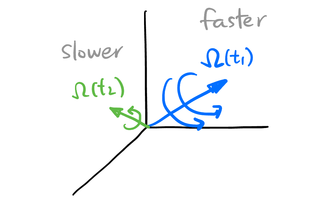
Compare this with how the angular velocity vector \(\boldsymbol{\Omega}\) encodes the rotation information: Figure 3.

Quick proof on the double covering

We will approach Equation 1 from the following simple steps:

1. Mental picture for the manifold \(SO(3)\): Three dimensional solid ball modulo the antipodal points on its surface: \[ SO(3) \simeq D^3/\sim \]

   

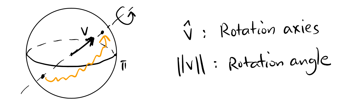
   Figure 1: Every point on \(D^3/\sim\) represent a rotation

2. Unit quaternions sits bijectively on the 3-sphere \(S^3\): \[ U(\mathbb{H}) \simeq \mathbb{S}^3. \]

   This is easy to see from the definition of unit quaternions: \[ \begin{aligned} U(\mathbb{H}) &:= \{ q \in \mathbb{H} : |q| = 1 \} \\ &\simeq \{ (a, b, c, d) \in \mathbb{R}^4 : a^2 + b^2 + c^2 + d^2 = 1 \} \\ &=: \mathbb{S}^3 \end{aligned} \] where \(q = a + b\mathbf{i} + c \mathbf{j} + d \mathbf{k}\).

3. Natural double cover projection from sphere to the equator plate: \[ \mathbb{S}^3 \overset{2:1} \twoheadrightarrow \frac{\mathbb{S}^3}{\sim} \simeq \frac{D^3}{\sim}. \]

   Just have a look at 2-dimensional case:

   

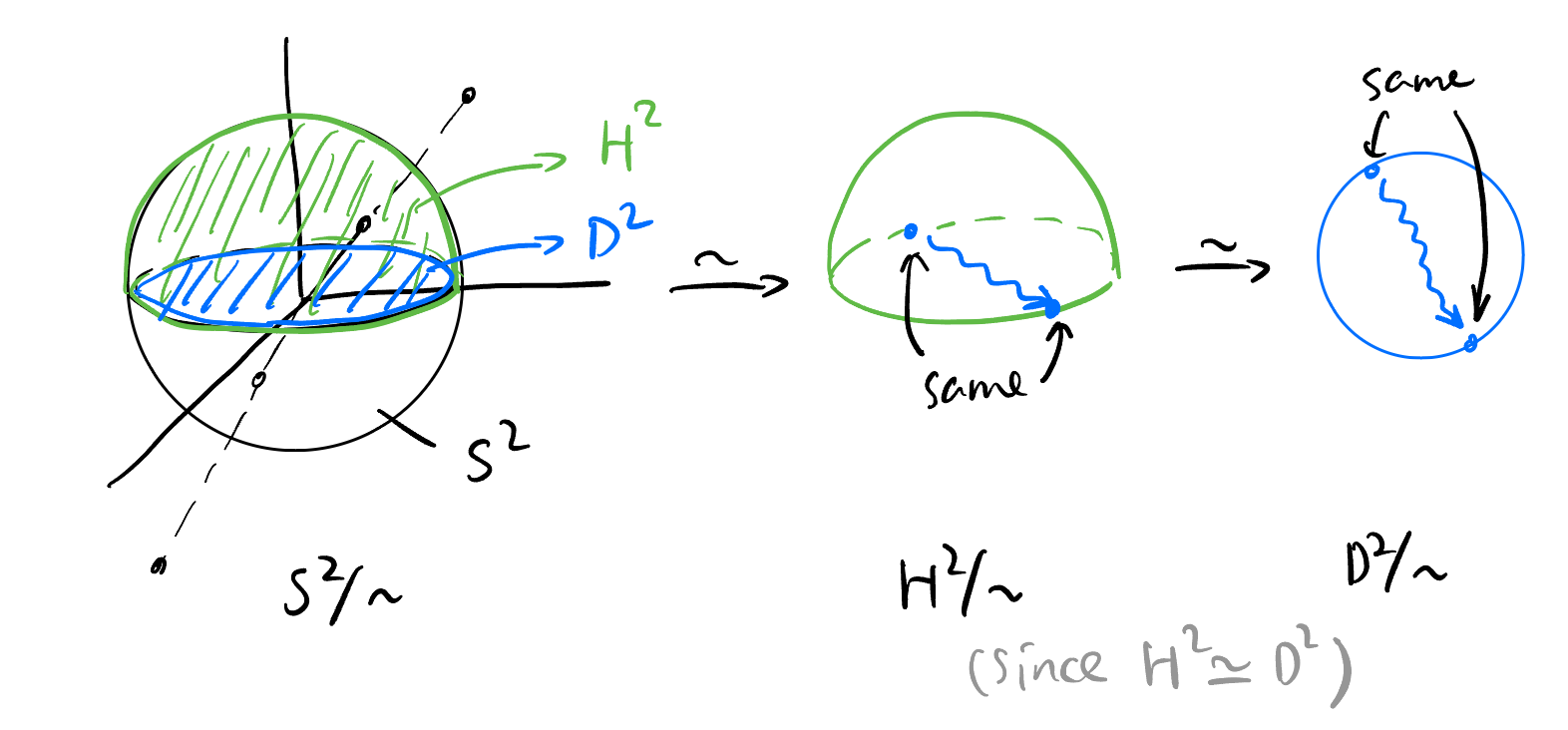
   Figure 2: 2-dimensional case of the natural double covering

4. From the above, we derived Equation 1.

1.2 Kinematics of rigid body: Quaternions version

Figure 3: How \(\boldsymbol{\Omega}(t)\) encodes the rotation axis and angular velocity

The time evolution of the attitude of a quadrocopter \(q(t)\) and the angular velocity vector¹ \(\boldsymbol{\Omega}(t)\) satisfy²: \[\dot{q} = \frac{1}{2} q \cdot \Omega. \tag{2}\]

¹ The angular velocity vector (shown in Figure 3) \(\boldsymbol{\Omega}(t_1) \in \mathbb{R}^3\) encodes the rotation axis (\(\boldsymbol{\hat{\Omega}}\)) and the angular velocity around that axis (\(\lVert\boldsymbol{\Omega}\rVert\)).

² You may be confused by how a quaternion could multiplied with a vector. It’s just because every vector \(v = v^1 \mathbf{i} + v^2 \mathbf{j} + v^3 \mathbf{k} \in \mathbb{R}^3\) naturally embedded into \(\mathbb{H}\) by a map \(p: \mathbb{R}^3 \to \mathbb{H}\), \(p(v) := 0 + v^1 \mathbf{i} + v^2 \mathbf{j} + v^3 \mathbf{k}\). Equation 2 is actually \(\dot{q} = \frac{1}{2} q \cdot p(\boldsymbol{\Omega})\).

Figure 4: Attitude of the quadrocopter as a path in \(D^3/\sim\)

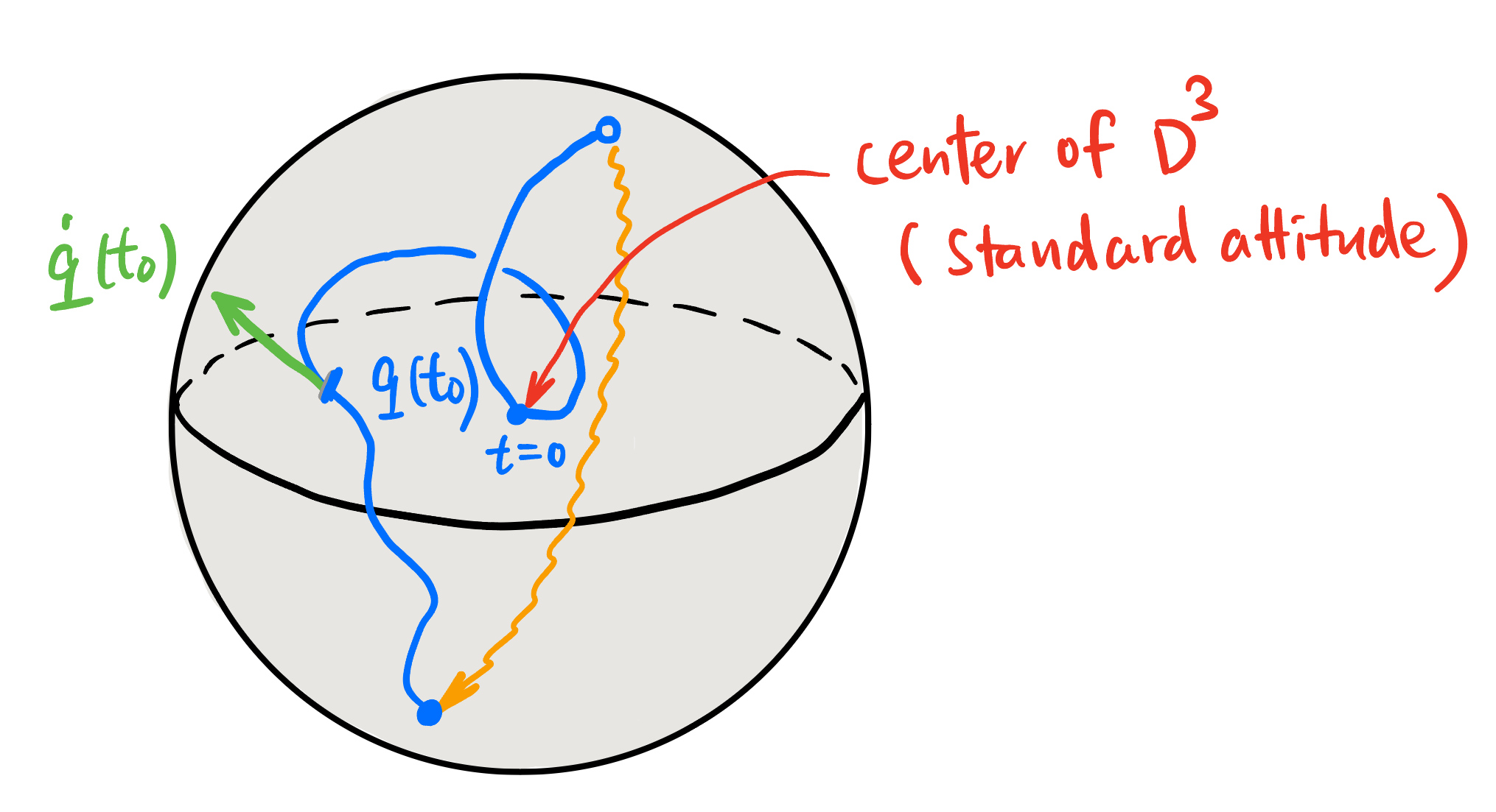
In other words, the attitude \(q(t)\) of a quadrocopter can be represented as a path in \(D^3 / \sim\) (shown in Figure 4), how to know the angular velocity vector \(\mathbf{\Omega}(t)\) at a time \(t_0\)? Equation 2 tells us just take the tangent vector (actually a quaternion \(\dot{q}\)) of the path at time \(t_0\), multiplied by 2 then divide by \(q\).

Proof of Equation 2

If both the attitude of the quadrocopter and the angular velocity vector is given at time \(t\), then the attitude configuration at time \(t + \Delta t\) can be determined and can be considered as the composition of two consecutive rotations:

• First, rotate the quadrocopter by \(q(t)\).
• Second, rotate the quadrocopter by a quaternion \(r(t)\) defined by \(\boldsymbol{\Omega}(t)\) and \(\Delta t\), which represents a small rotation (where \(\Delta \theta\) is a small angle around the axis \(\hat{\Omega}(t)\)): \[ \begin{aligned} r(t) &= \cos\left(\frac{\Delta \theta}{2}\right) + \sin\left(\frac{\Delta \theta}{2}\right) \hat{\Omega}(t) \\ &= \cos\left(\frac{\lVert\boldsymbol{\Omega}(t)\rVert \Delta t}{2}\right) + \sin\left(\frac{\lVert\boldsymbol{\Omega}(t)\rVert \Delta t}{2}\right) \hat{\Omega}(t). \end{aligned} \]

Therefore, the attitude at time \(t + \Delta t\) can be expressed as³: \[ \begin{align*} &\begin{aligned} q(t + \Delta t) &= q(t) \cdot r(t) \\ &= q(t) \cdot \left( \cos\left(\frac{\lVert\boldsymbol{\Omega}(t)\rVert \Delta t}{2}\right) + \sin\left(\frac{\lVert\boldsymbol{\Omega}(t)\rVert \Delta t}{2}\right) \hat{\Omega}(t) \right) \\ &= q(t) \cdot \left( 1 + \frac{\lVert\boldsymbol{\Omega}(t)\rVert \Delta t}{2} \frac{\Omega(t)}{\lVert\boldsymbol{\Omega}(t)\rVert} \right) + o(\Delta t) \quad \text{(First order approximation)} \end{aligned} \\ \implies\quad & \frac{q(t + \Delta t) - q(t)}{\Delta t} \approx \frac{1}{2} q(t) \cdot \Omega(t) \\ \implies\quad & \dot{q}(t) = \frac{1}{2} q(t) \cdot \Omega(t). \end{align*} \]

We are done!

³ In this post, \(q \cdot p\) reads from left to right, i.e., \(q\) is rotated first and then \(p\).

Q&A for Equation 2

1. Q1: The attitude of the quadrocopter can be represented by two quaternions \(\pm q \in U(\mathbb{H})\), but there’s only one possible \(\mathbf{\Omega}(t)\) at a given time. Why?

   A1: Both \(q\) and \(-q\) satisfy Equation 2 with the same \(\mathbf{\Omega}(t)\): \[ \begin{aligned} \frac{\mathrm{d}}{\mathrm{d} t} q &= \frac{1}{2} q \cdot \Omega \\ \frac{\mathrm{d}}{\mathrm{d} t} (-q) &= \frac{1}{2} (-q) \cdot \Omega \end{aligned} \]

2. Q2: Given any path⁴ \(q(t)\) in \(D^3/\sim\), the angular velocity vector can be computed by: \[ \Omega = 2 \frac{\dot{q}}{q}. \] Does this result \(\Omega\) guaranteed to be purely imaginary? (Because angular velocity vector must be purely imaginary).

   A2: Yes. We give the following theorems first:

Quaternion product rule

Theorem 1 Let quaternions \[ \begin{aligned} p &\equiv a + \mathbf{u}, \\ q &\equiv b + \mathbf{v}. \end{aligned} \]

Their product is given by: \[ p \cdot q = ab - \mathbf{u} \cdot \mathbf{v} + a \mathbf{v} + b \mathbf{u} + \mathbf{u} \times \mathbf{v}. \]

Inner product in \(\mathbb{H}\)

Theorem 2 Since \(\mathbb{H} \simeq \mathbb{R}^4\) as vector spaces, we can borrow the inner product structure on \(\mathbb{R}^4\) to \(\mathbb{H}\). Let \(p, q \in \mathbb{H}\), define: \[ \langle p, q \rangle = \sum_{i=0}^3 p_i q_i. \] Also we have: \[ \Re(p \cdot q) = \langle p, \bar{q} \rangle = \langle \bar{p}, q \rangle. \]

Proof of Theorem 2

By Theorem 1, \[ \begin{aligned} \Re(p \cdot q) &= \Re(\overbrace{ab - \mathbf{u} \cdot \mathbf{v}}^{\text{scalar}} + \overbrace{a \mathbf{v} + b \mathbf{u} + \mathbf{u} \times \mathbf{v}}^{\text{vector}}) \\ &= ab - \mathbf{u} \cdot \mathbf{v} \\ &= p_0 q_0 - p_1 q_1 - p_2 q_2 - p_3 q_3 \\ &= \langle p, \bar{q} \rangle \\ &= \langle \bar{p}, q \rangle. \end{aligned} \]

Remember \(q(t)\) also lives on the surface \(\mathbb{S}^3\), so: \[ \frac{\dot{q}}{q} = \dot{q} \bar{q}. \]

Since \(\dot{q}(t)\) is a tangent vector to the surface \(\mathbb{S}^3\), \(\dot{q} \perp q\) as vectors in \(\mathbb{R}^4\), i.e., \[ \langle \dot{q}, q \rangle = 0. \] By Theorem 2, \[ \langle \dot{q}, q \rangle = \Re (\dot{q} \cdot \bar{q}) = 0, \] i.e., \[ \Re (\Omega) = 0. \]

So \(\Omega\) is purely imaginary. Done!

⁴ Any path in \(D^3/\sim\) is a legitimate attitude change of the quadrocopter.

The rest content may contain some errors, please be careful when reading.

2 Model

2.1 Dynamics Equations without thrust

The dynamics \(\dot{\mathbf{x}} = \phi(\mathbf{x})\) is given by:

Position dynamics:

\[\dot{\mathbf{r}} = \mathbf{v}\]

Velocity dynamics (Newton’s second law with only gravity):

\[\dot{\mathbf{v}} = -g\mathbf{e}_3\]

Orientation dynamics (quaternion kinematics):

\[\dot{q} = \frac{1}{2}q \cdot p(\boldsymbol{\Omega})\]

As shown in equation (20) of the paper:

\[\dot{q} = \begin{pmatrix} \dot{q}_0 \\ \dot{q}_{1:3} \end{pmatrix} = \frac{1}{2} \begin{pmatrix} -q_{1:3}^T\boldsymbol{\Omega} \\ (S(q_{1:3}) + q_0\mathbf{I})\boldsymbol{\Omega} \end{pmatrix}\]

Where \(S(q1:3)S(q_{1:3}) S(q1:3​)\) is the skew-symmetric matrix:

\[S(q_{1:3}) = \begin{pmatrix} 0 & -q_3 & q_2 \\ q_3 & 0 & -q_1 \\ -q_2 & q_1 & 0 \end{pmatrix}\]

Angular velocity dynamics (Euler’s equations without external torques):

\[\dot{\boldsymbol{\Omega}} = -\mathbf{J}^{-1}(\boldsymbol{\Omega} \times (\mathbf{J}\boldsymbol{\Omega}))\]

\[\dot{\mathbf{x}} = \phi(\mathbf{x}) = \begin{pmatrix} \mathbf{v} \ -g\mathbf{e}_3 \ \frac{1}{2}q \cdot p(\boldsymbol{\Omega}) \ -\mathbf{J}^{-1}(\boldsymbol{\Omega} \times (\mathbf{J}\boldsymbol{\Omega})) \end{pmatrix}\]

It’s worth noting that this represents the dynamics of a free-falling quadrocopter with no thrust forces (as the human specified “without control”). In reality, even in a passive state, a quadrocopter would have some baseline thrust from spinning propellers. For a more realistic “passive” model, we could include a constant collective thrust ff f acting along the body’s z-axis, which would modify the velocity dynamics to:

\[ \dot{\mathbf{v}} = -g \mathbf{e}_3 + \frac{f}{m} R(q) \mathbf{e}_3 \]

Where \(R(q)\) is the rotation matrix corresponding to quaternion \(q\).

These equations capture the full nonlinear dynamics of the quadrocopter in phase space, representing how position, velocity, orientation, and angular velocity evolve over time in the absence of control inputs.

3 Quadrocopter Dynamics with Motor Control in Phase Space

3.1 State Vector and Basic Parameters

As before, the state vector in phase space is: \[\mathbf{x} = (\mathbf{r}, \mathbf{v}, q, \boldsymbol{\Omega})\]

Where: - \(\mathbf{r} \in \mathbb{R}^3\) is the position in inertial frame - \(\mathbf{v} \in \mathbb{R}^3\) is the linear velocity in inertial frame - \(q \in \mathbb{S}^3\) is the unit quaternion representing orientation - \(\boldsymbol{\Omega} \in \mathbb{R}^3\) is the angular velocity vector in body frame

3.2 Motor and Physical Parameters

• \(m\): mass of the quadrocopter
• \(\mathbf{J} \in \mathbb{R}^{3 \times 3}\): inertia tensor (typically diagonal for a symmetric quadrocopter)
• \(g\): gravitational acceleration (9.81 m/s²)
• \(L\): distance from center of mass to each motor (arm length)
• \(k_T\): thrust coefficient (converts squared motor speed to thrust force)
• \(k_M\): moment coefficient (relates thrust to reactive torque)
• \(\omega_i\): angular velocity of motor \(i\) for \(i \in \{1,2,3,4\}\)
• \(\mathbf{e}_3 = (0,0,1)^T\): unit vector in the z-direction

3.3 Motor Forces and Torques

Each motor produces: - Thrust force: \(F_i = k_T\omega_i^2\) - Reactive torque: \(M_i = k_M\omega_i^2\)

For a typical “+” configuration (1-front, 2-right, 3-back, 4-left):

1. Total thrust: \(F = \sum_{i=1}^4 F_i = k_T\sum_{i=1}^4 \omega_i^2\)

2. Moment vector in body frame: \[\boldsymbol{\tau} = \begin{pmatrix} \tau_x \\ \tau_y \\ \tau_z \end{pmatrix} = \begin{pmatrix} L(F_4 - F_2) \\ L(F_1 - F_3) \\ M_1 - M_2 + M_3 - M_4 \end{pmatrix}\]

   Substituting motor forces: \[\boldsymbol{\tau} = \begin{pmatrix} Lk_T(\omega_4^2 - \omega_2^2) \\ Lk_T(\omega_1^2 - \omega_3^2) \\ k_M(\omega_1^2 - \omega_2^2 + \omega_3^2 - \omega_4^2) \end{pmatrix}\]

3.4 Control Input Mapping

We can define a mapping from motor speeds to control inputs: \[\begin{pmatrix} F \\ \tau_x \\ \tau_y \\ \tau_z \end{pmatrix} = \begin{pmatrix} k_T & k_T & k_T & k_T \\ 0 & -Lk_T & 0 & Lk_T \\ Lk_T & 0 & -Lk_T & 0 \\ k_M & -k_M & k_M & -k_M \end{pmatrix} \begin{pmatrix} \omega_1^2 \\ \omega_2^2 \\ \omega_3^2 \\ \omega_4^2 \end{pmatrix}\]

3.5 Dynamics Equations with Control

1. Position dynamics: \[\dot{\mathbf{r}} = \mathbf{v}\]

2. Velocity dynamics (with thrust force): \[\dot{\mathbf{v}} = -g\mathbf{e}_3 + \frac{F}{m}R(q)\mathbf{e}_3\]

   Where \(R(q)\) is the rotation matrix corresponding to quaternion \(q\), which transforms the body-fixed thrust direction to the inertial frame.

3. Orientation dynamics (quaternion kinematics): \[\dot{q} = \frac{1}{2}q \cdot p(\boldsymbol{\Omega})\]

   As expressed in component form: \[\dot{q} = \begin{pmatrix} \dot{q}_0 \\ \dot{q}_{1:3} \end{pmatrix} = \frac{1}{2} \begin{pmatrix} -q_{1:3}^T\boldsymbol{\Omega} \\ (S(q_{1:3}) + q_0\mathbf{I})\boldsymbol{\Omega} \end{pmatrix}\]

   Where \(S(q_{1:3})\) is the skew-symmetric matrix of the vector part of the quaternion.

4. Angular velocity dynamics (Euler’s equations with motor torques): \[\dot{\boldsymbol{\Omega}} = \mathbf{J}^{-1}(\boldsymbol{\tau} - \boldsymbol{\Omega} \times (\mathbf{J}\boldsymbol{\Omega}))\]

3.6 Complete System Dynamics

The full dynamics of the controlled quadrocopter in phase space are:

\[\dot{\mathbf{x}} = \phi(\mathbf{x}, \mathbf{u}) = \begin{pmatrix} \mathbf{v} \\ -g\mathbf{e}_3 + \frac{F}{m}R(q)\mathbf{e}_3 \\ \frac{1}{2}q \cdot p(\boldsymbol{\Omega}) \\ \mathbf{J}^{-1}(\boldsymbol{\tau} - \boldsymbol{\Omega} \times (\mathbf{J}\boldsymbol{\Omega})) \end{pmatrix}\]

Where the control input \(\mathbf{u} = (\omega_1^2, \omega_2^2, \omega_3^2, \omega_4^2)\) represents the squared motor speeds.

These nonlinear differential equations fully describe the quadrocopter’s motion under motor control, capturing the complex interactions between thrust forces, aerodynamic torques, and rigid body dynamics.

Note that in practice, there may be additional terms for aerodynamic drag, motor dynamics, and other effects, but this model captures the essential physics of quadrocopter flight with motor control.