Basics of Projective Space and Projective Linear Group 射影空间与射影线性群
1 Projective Space
1.1 Intuition
The projective space of a vector space is the set of all lines1 through the origin with some extra structures.
1 Or “1-dimensional subspaces”.
1.2 Definition
This can be formally defined by identifying some elements in a vector space \(V\), or classifying the vectors in \(V\) according to the spaces they span. This is exactly the idea of “quotients” in math.
2 \(\mathbb{F}^* := \mathbb{F} - \{0_\mathbb{F}\}\), i.e., the non-zero elements of the field \(\mathbb{F}\).
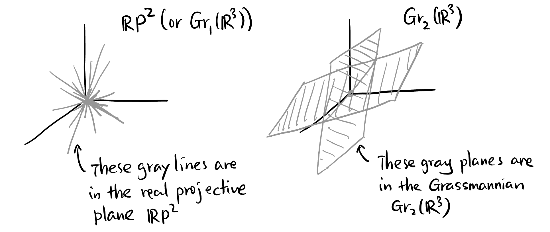
All \(1\)-dimensional subspaces form the projective space. What about \(n\)-dimensional subspaces? They form the so-called Grassmannian manifold!
1.3 Canonical projection
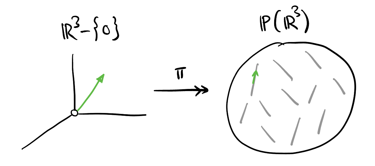
There is a (surjective) canonical projection \[ \begin{aligned} \pi: V - \{0_V\} &\twoheadrightarrow \mathbb{P}(V) \\ x &\mapsto [x]_{\sim} \end{aligned} \] that maps each non-zero vector to its equivalence class (as shown in Figure 2).
In the following post, we will only consider the case where \(\mathbb{F} \in \{\mathbb{R}, \mathbb{C}\}\) and \(V = \mathbb{F}^n\) since they are the most common cases that we will encounter. It’s necessary to have a clear mental picture of each of the example in the following sections.
2 Real Projective Space \(\mathbb{RP}^n\)
When \(V = \mathbb{R}^n\), we will denote \(\mathbb{P}(\mathbb{R}^n)\) by \(\mathbb{RP}^{n-1}\), where the upper index indicates the dimension of the projective space (actually a manifold of dimension \(n-1\)).
The “shape” of \(\mathbb{RP}^n\) can be understood by Equation 1.
\[ \boxed{ \mathbb{RP}^n \simeq \frac{\mathbb{S}^n}{\mathbb{Z}_2} \simeq \frac{H^n}{\sim} \simeq \frac{D^n}{\sim}. } \tag{1}\]
This is a diffeomorphism in the category of smooth manifolds.
The notations in Equation 1 are defined below:
\(\mathbb{S}^n\) is the \(n\)-dimensional sphere: \[ \mathbb{S}^n := \{x \in \mathbb{R}^{n+1} : \|x\| = 1\}. \]
\(H^n\) is the upper hemisphere: \[ H^n := \{x \in \mathbb{R}^{n+1} : \|x\| = 1, x_j \geq 0\}, \] where \(j\) can be any coordinate index of \(x\).
\(D^n\) is the closed \(n\)-disk: \[ D^n := \{x \in \mathbb{R}^{n} : \|x\| \leq 1\}. \]
\(\mathbb{S}^n/\mathbb{Z}_2\) means:
\[ \mathbb{S}^n/\text{\{antipodal points\}} \] Let the group \(\mathbb{Z}/2\mathbb{Z} = \{\bar{0}, \bar{1}\}\) acts on \(\mathbb{S}^n\) by taking the antipodal point: \[ \bar{1} \cdot x = -x, \quad \forall x \in \mathbb{S}^n. \] This action defines the equivalence relation (See wiki here): \[ \forall x \in \mathbb{S}^n, x \sim y :\iff \exists \lambda \in \mathbb{Z}_2, y = \lambda x. \]
The equivalence relation \(\sim\) on \(H^n\) is defined as: \[ \forall x, y \in H^n, x \sim y :\iff x = y \text{ or } \begin{cases} x, y \in \partial H^n = \mathbb{S}^{n-1}, \\ x=-y. \end{cases} \]
The equivalence relation \(\sim\) on \(D^n\) is defined as: \[ \forall x, y \in D^n, x \sim y :\iff x = y \text{ or } \begin{cases} x, y \in \partial D^n = \mathbb{S}^{n-1}, \\ x=-y. \end{cases} \]
This is explained in detail below.
2.1 Real Projective line3 \(\mathbb{RP}^1\)
Let \(V = \mathbb{R}^2\), then4: \[ \mathbb{RP}^1 \simeq \frac{\mathbb{S}^1}{\mathbb{Z}_2} \simeq \frac{H^1}{\sim} \simeq \frac{D^1}{\sim} \simeq \mathbb{S}^1 \simeq \mathbb{\hat{R}}. \tag{2}\]
4 \(\mathbb{\hat{R}} := \mathbb{R} \cup \{\infty\}\) is called the projectively extended real line. Distinguish it from the extended real line \(\overline{\mathbb{R}} := \mathbb{R} \cup \{-\infty, +\infty\}\).
5 The blue curly arrow in Figure 3 indicates that the two points are equivalent. One can be immediately transported to the other side by this arrow.
Visually speaking5,
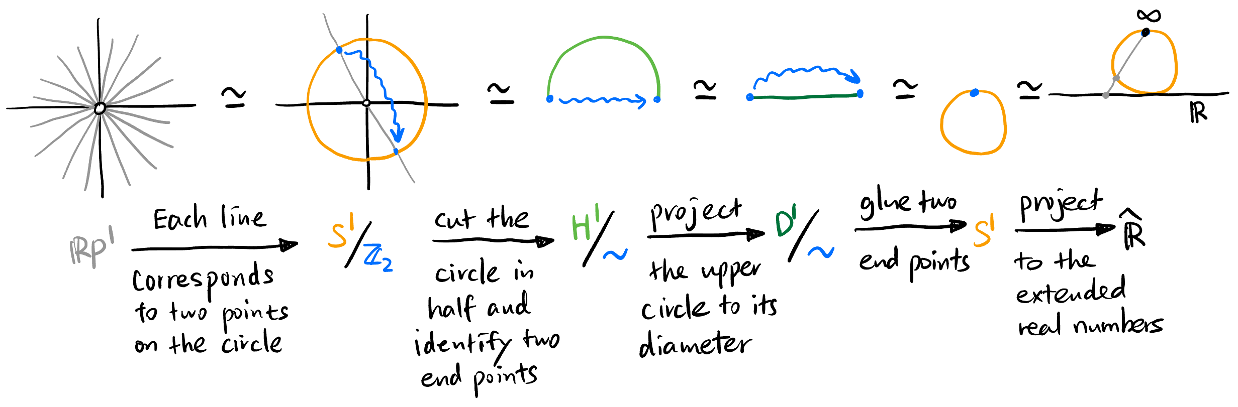
Note that in Equation 2, \(D^1/{\sim}\) happens to be \(\mathbb{S}^1\) again, which is very special and not general for \(n > 1\).
Instead of let a line intersects the unit circle at the origin (as shown in the first isomorphism in Equation 2), there are different graphical representations of \(\mathbb{RP}^1\):
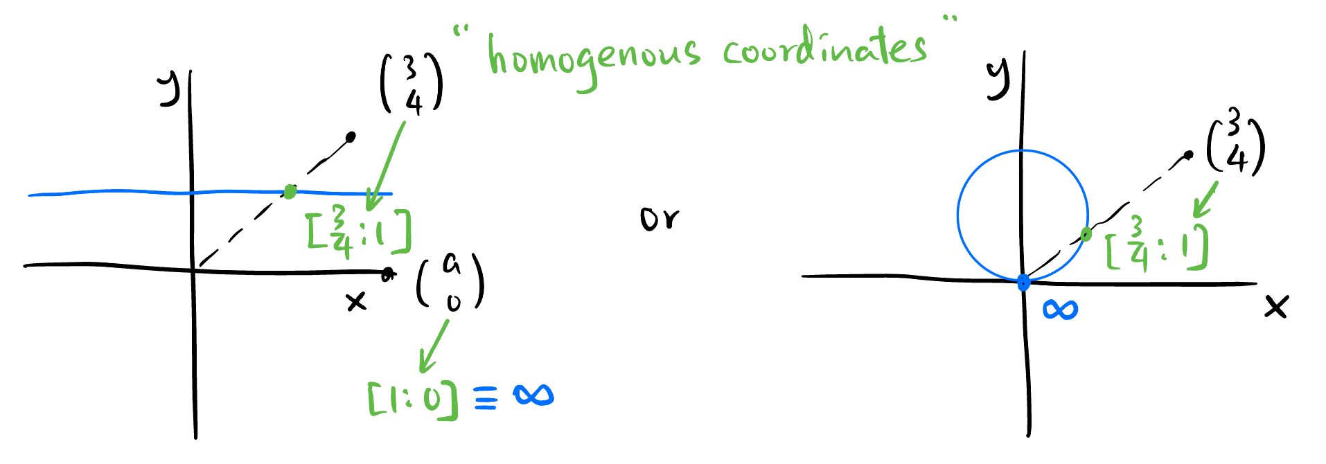
The horizontal line in Figure 4 does not intersect the blue line. We thus define it belongs to the equivalent class \(\{\infty\}\).
3 The projective space for \(V = \mathbb{R}^1\) is too trivial, since everything in \(\mathbb{R}\) is in one equivalence class. Therefore, \(\mathbb{RP}^0 = \{e\}\).
2.2 Real Projective plane \(\mathbb{RP}^2\)
Let \(V = \mathbb{R}^3\), then: \[ \mathbb{RP}^2 \simeq \frac{\mathbb{S}^2}{\mathbb{Z}_2} \simeq \frac{H^2}{\sim} \simeq \frac{D^2}{\sim}. \tag{3}\]
Visually speaking,
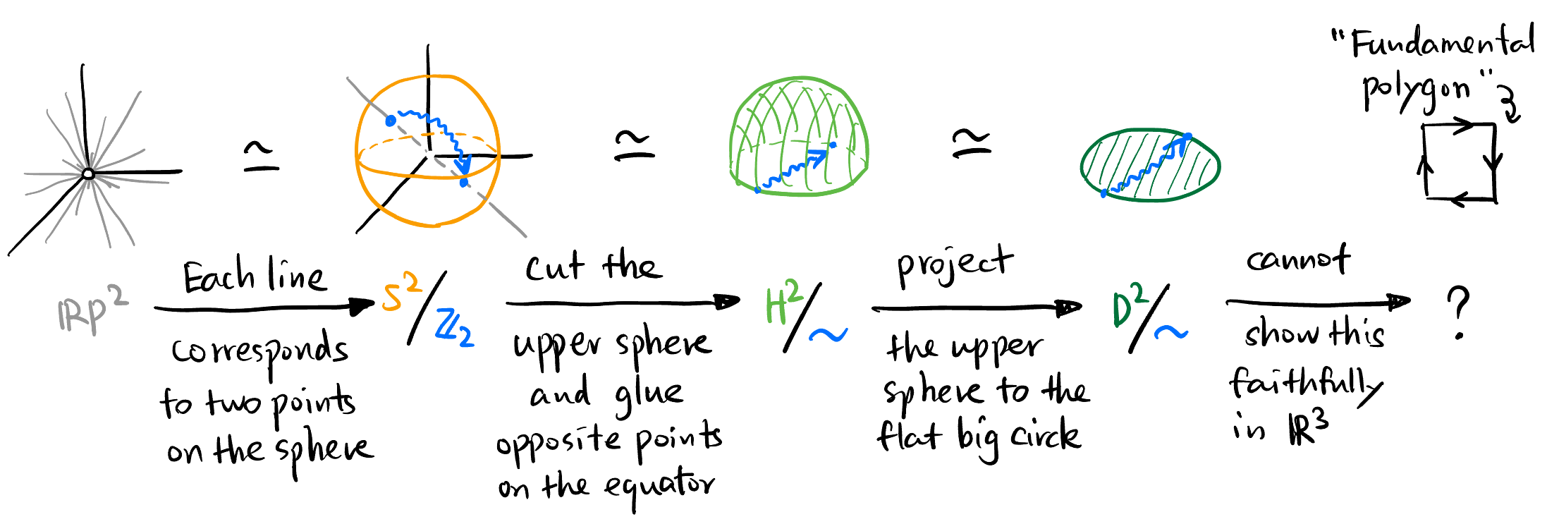
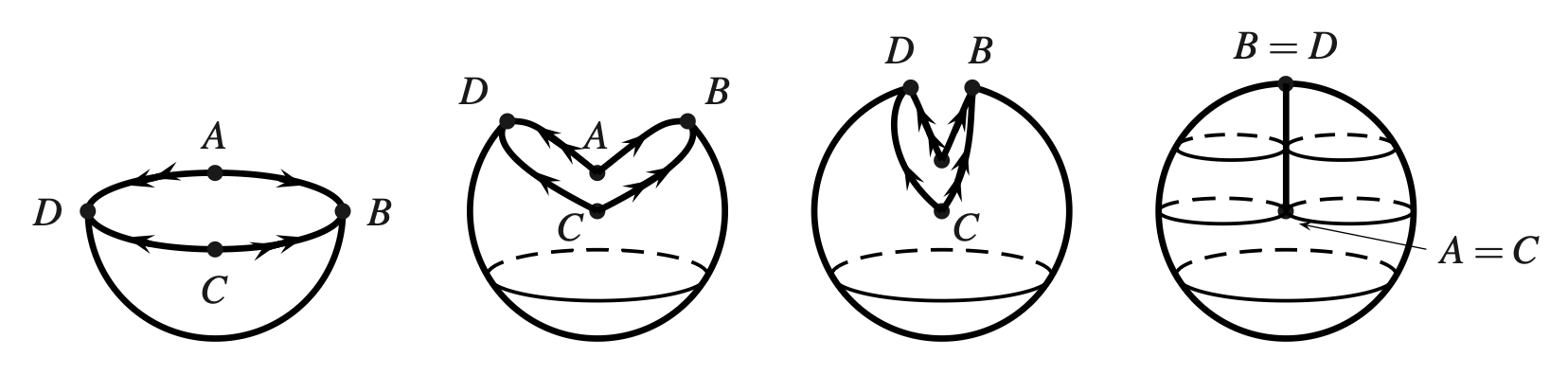
Note that we cannot glue the opposite points on \(H^2\) nor \(D^2\) in \(\mathbb{R}^3\) without a self-intersection. So we ended up at \(D^2/{\sim}\). This structure is often expressed using fundamental polygon. Figure 6 [1] is what you get if you force to glue the opposite points on the equator of \(H^2\) together.
Instead of let a line intersects the unit sphere at the origin (as shown in the first isomorphism in Equation 3), there are a different graphical representation of \(\mathbb{RP}^2\):
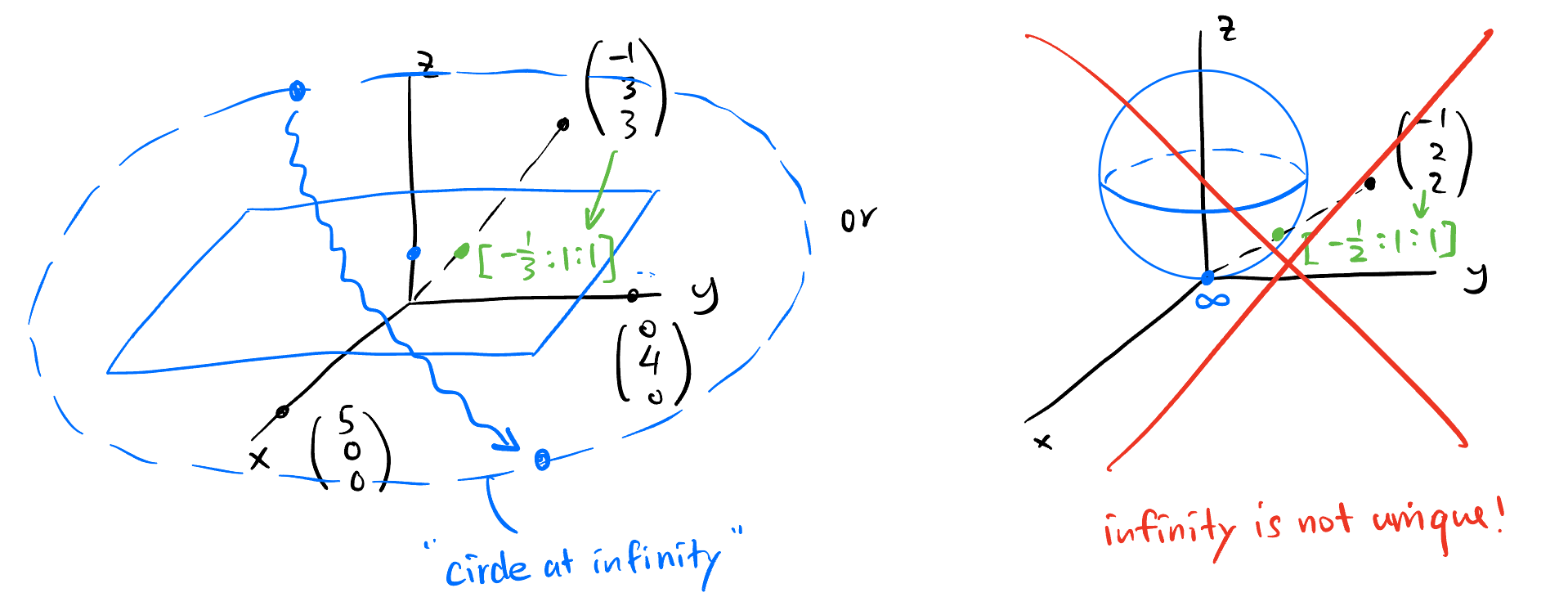
The lines in the \(xy\) plane in Figure 7 do not intersect the blue plane. We thus define them to “intersect with the circle at infinity”. The right figure of Figure 7 is NOT true since there is only one infinity, so it cannot tell the difference of the lines in the \(xy\) plane. So notably, \[ \begin{aligned} \mathbb{RP}^2 &\simeq \mathbb{R}^2 \cup \{\text{circle at infinity}\} \\ &\not\simeq \mathbb{R}^2 \cup \{\infty\}. \end{aligned} \]
2.3 Real Projective space \(\mathbb{RP}^3\)
Let \(V = \mathbb{R}^4\), one could prove that Equation 1 is still symbolically true: \[ \mathbb{RP}^3 \simeq \frac{\mathbb{S}^3}{\mathbb{Z}_2} \simeq \frac{H^3}{\sim} \simeq \frac{D^3}{\sim}. \tag{4}\]
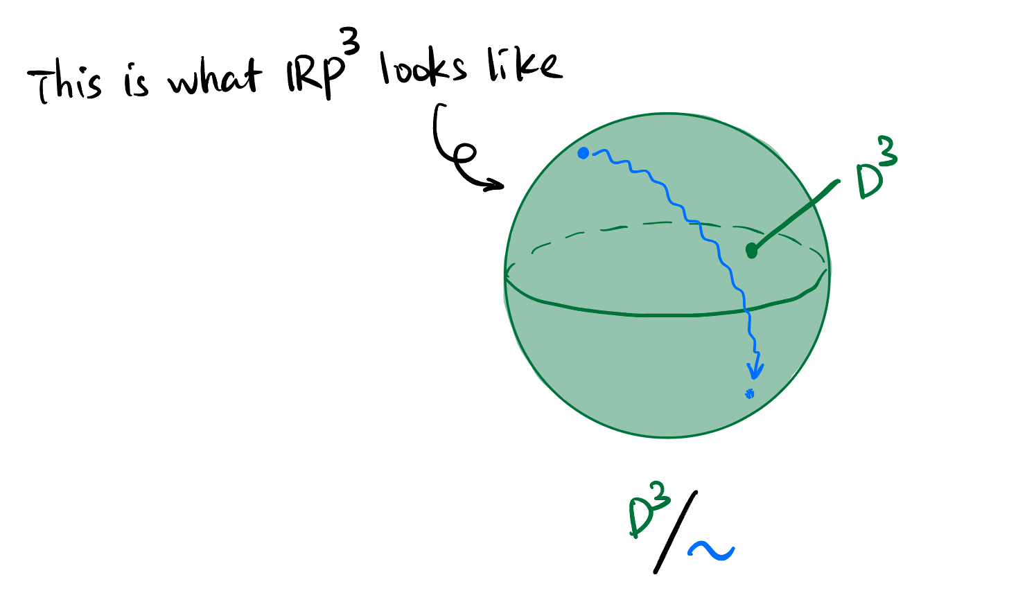
However this time, the only object in Equation 4 that can be visualized is \(D^3/{\sim}\):
Their relations are: \[ \boxed{ \text{Spin}(3) \simeq SU(2) \simeq \mathbb{S}^3 \simeq U(\mathbb{H}) \overset{2:1} \twoheadrightarrow \mathbb{RP}^3 \simeq SO(3). } \]
- \(SU(2) \simeq \mathbb{S}^3\): Rotation in \(\mathbb{C}^2\) sits bijectively on the surface of the 3-sphere \(S^3\).
- \(\mathbb{S}^3 \simeq U(\mathbb{H})\): Unit quaternions live on the 3-sphere.
- \(\mathbb{RP}^3 \simeq SO(3)\): If you look around in \(\mathbb{R}^4\), what you see is rotations in \(\mathbb{R}^3\)!
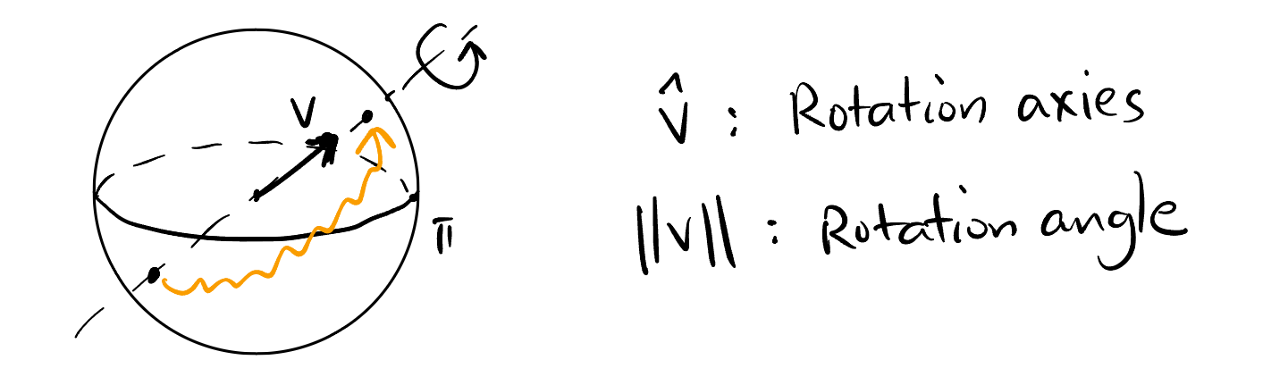
An element \(R \in SO(3)\) is specified by the rotation axis and the rotation angle. We could encode these two information by a single vector in a solid ball of radius \(\pi\), where the length of \(V\) is the rotation angle and the direction of \(V\) is the rotation axis. However, we soon realize that antipodal points on the surface of \(D^3\) represent the same rotation since rotating by \(\pi\) does not care about the rotation direction. So we end up with the quotient space \(D^3/{\sim}\) (shown in Figure 9).
But Figure 9 is also the space of \(\mathbb{RP}^3\), so we get: \[ \mathbb{RP}^3 \simeq SO(3). \]
- \(\mathbb{S}^3 \overset{2:1}{\twoheadrightarrow} SO(3)\): A rotation in \(\mathbb{R}^3\) is represented by two points on the 3-sphere.
- \(\text{Spin}(3) \simeq \mathbb{S}^3\): Spin group double covers the rotation group.
3 Complex Projective Space \(\mathbb{CP}^n\)
We don’t have a formula like Equation 1 for \(\mathbb{CP}^n\) by the way. We will only focus on one case where \(V = \mathbb{C}^2\).
3.1 Complex projective line6 \(\mathbb{CP}^1\)
Let \(V = \mathbb{C}^2\). Although it’s impossible to have a mental picture of \(\mathbb{C}^2\), we could have a legit imagination for \(\mathbb{CP}^1\) using homogeneous coordinates: \[ \mathbb{C}^2 - \{0\} \ni \begin{pmatrix} z_1 \\ z_2 \\\end{pmatrix} \xmapsto{\pi} \left[\frac{z_1}{z_2} : 1\right] \equiv \left[a+bi : 1\right] \simeq \mathbb{C}. \tag{5}\]
According to Equation 5, one would need one single complex number \(a+bi\) to specify an element in \(\mathbb{CP}^1\). Does it implies that \(\mathbb{CP}^1\) is just the complex line7? No! We missed the case where \(z_2 = 0\)! Similar to Section 2.1, we define the line \(\begin{pmatrix} z_1 \\ 0 \\\end{pmatrix} \in \mathbb{C}^2 - \{0\}\) belongs to the equivalence class denoted by the symbol \(\infty\): \[ \begin{pmatrix} z_1 \\ 0 \\\end{pmatrix} :\xmapsto{\pi} \left[1 : 0\right] \equiv \infty \]
7 \(\mathbb{C}\) has different dimension as a real or complex vector space: \[\operatorname{dim}_{\mathbb{R}} \mathbb{C} = 2, \operatorname{dim}_{\mathbb{C}} \mathbb{C} = 1.\] We consider \(\mathbb{C}\) as a complex vector space here, so we call it the complex line instead of the complex plane.
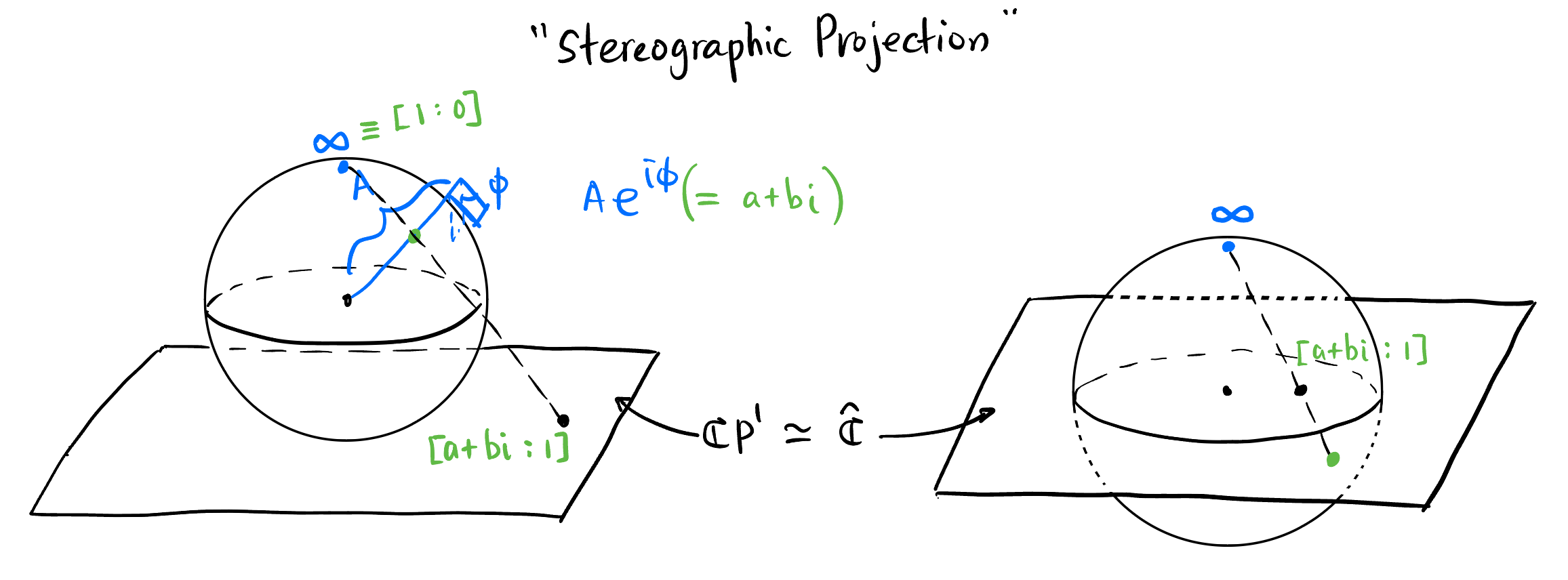
Therefore, we would need one complex number plus only one extra symbol \(\infty\) (together called the projectively extended complex number \(\mathbb{\hat{C}}\)) to specify an element in \(\mathbb{CP}^1\): \[ \mathbb{CP}^1 \simeq \mathbb{C} \cup \{\infty\} \equiv \mathbb{\hat{C}}. \]
We could also put a 2-sphere across or above \(\mathbb{\hat{C}}\) (as shown in Figure 10) and construct a bijective correspondence (called the Stereographic projection) between the points on the sphere and the points on \(\mathbb{\hat{C}}\). This sphere is a compact, connected, 1-dimensional complex manifold, called the Riemann sphere. We have the isomorphism: \[ \mathbb{CP}^1 \simeq \mathbb{S}^2. \]
6 The projective space for \(V = \mathbb{C}^1\) is too trivial, since everything in \(\mathbb{C}\) is in one equivalence class. Therefore, \(\mathbb{CP}^0 = \{e\}\).
4 Homography
Whenever mathematicians define a new object, they will soon talk about the morphisms between them, i.e., the mappings that preserve the structures of the objects. We are interested specifically in bijective morphisms between projective spaces, which are called homography. Just like the general linear group \(\text{GL}(V)\), all homographies form a group called the projective linear group \(\text{PGL}(V)\).
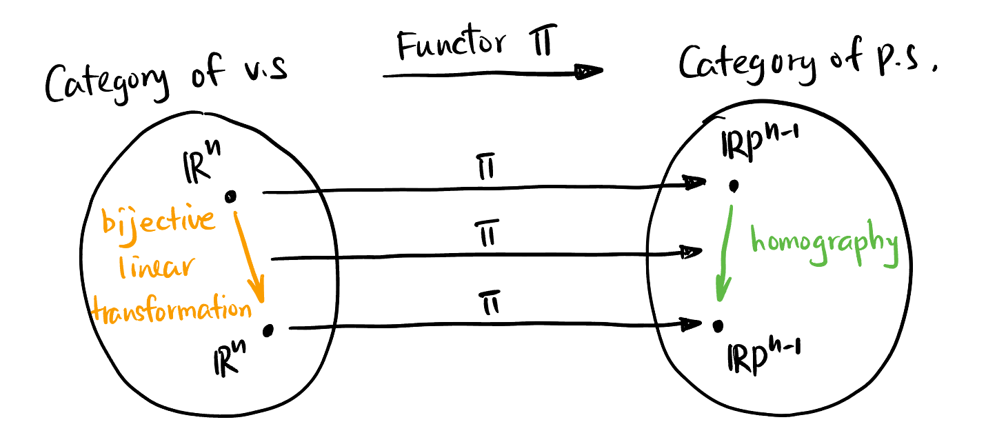
Homography is an isomorphism between projective spaces induced by bijective linear transformations of vector spaces. \[\text{PGL}(V) \equiv \operatorname{Aut}(\mathbb{P}(V)).\]
The canonical projection \(\pi\) in Section 1.3 not only project vector spaces but also the linear transformations between vector spaces. So it could be viewed as a functor from the category of vector spaces (v.s.) to the category of projective spaces (p.s.):
We first give two examples of homography in the case of \(V \in \{\mathbb{R}^2, \mathbb{C}^2\}\) before dealing with the case of abstract \(V\).
4.1 Homography on \(\mathbb{RP}^1\)
Let \(V = \mathbb{R}^2, A \in \text{GL}(V)\), what is \(A\) under the functor \(\pi\)?
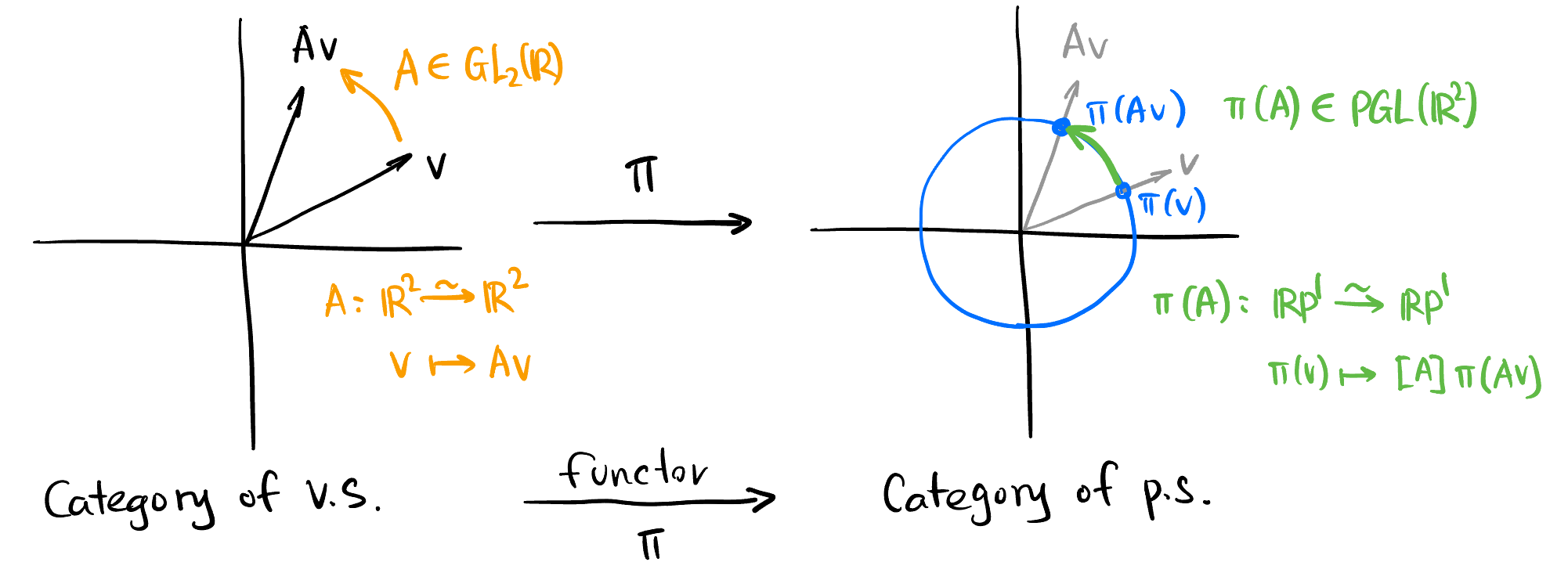
\(A\) could be represented by a \(2 \times 2\) non-singular matrix multiplied by a non-zero vector \(v\): \[ \begin{aligned} A: \mathbb{R}^2 &\xrightarrow[]{\sim} \mathbb{R}^2 \\ \begin{pmatrix} x_0 \\ y_0 \\\end{pmatrix} &\mapsto \begin{pmatrix} a & c \\ b & d \\\end{pmatrix} \begin{pmatrix} x_0 \\ y_0 \\\end{pmatrix}\\ \begin{pmatrix} x \\ 1 \\\end{pmatrix} &\mapsto \begin{pmatrix} a & c \\ b & d \\\end{pmatrix} \begin{pmatrix} x \\ 1 \\\end{pmatrix} = \begin{pmatrix} ax + c \\ bx + d \\\end{pmatrix} \end{aligned} \] where \(x \in \mathbb{\hat{R}}\), \(x_0, y_0, a, b, c, d \in \mathbb{R}\) and \(ad-bc \neq 0\). By definition, \(\pi(A)\) should map the equivalence class \([x : 1]\) to \([ax + c : bx + d]\): \[ \begin{aligned} \pi(A): \mathbb{RP}^1 &\xrightarrow[]{\sim} \mathbb{RP}^1 \\ [x : 1] &\mapsto \left[\frac{ax+c}{bx+d} : 1\right] \\ \end{aligned} \tag{6}\]
Note that \(\pi(A)\) maps \(\infty\) to \(\frac{a}{b}\).
4.2 Möbius transformations – Homography on \(\mathbb{CP}^1\)
Homographies on \(\mathbb{CP}^1\) are called Möbius transformations. The object \(\text{PGL}(\mathbb{C}^2)\) is called the Möbius group.
Let \(V = \mathbb{C}^2, A \in \text{GL}(V)\). We could simply write Equation 6 as its complex version: \[ \begin{aligned} \pi(A): \mathbb{CP}^1 &\xrightarrow[]{\sim} \mathbb{CP}^1 \\ [z : 1] &\mapsto \left[\frac{az+c}{bz+d} : 1\right] \\ \end{aligned} \] where \(z \in \mathbb{\hat{C}}\), \(a, b, c, d \in \mathbb{C}\) and \(ad-bc \neq 0\). Also, \(\pi(A)\) maps \(\infty\) to \(\frac{a}{b}\).
There is an astounding fact [2] that the elements in the Möbius group correspond bijectively to the rigid motions of the Riemann sphere.
However, this does NOT mean that \(\text{PGL}(\mathbb{C}^2) \simeq SO(3)\) as groups. In fact, one can show that the Möbius group is isomorphic to the so-called Lorenz group: \[ \text{PGL}(\mathbb{C}^2) \simeq SO^+(1, 3). \]
5 Projective Linear group
The projective space is a classification of vectors in a vector space. Similarly, we will define the projective linear group \(\text{PGL}(V)\) as a classification of isomorphisms in the general linear group \(\text{GL}(V)\) in this section.
5.1 Definition
It’s obvious that some linear transformations are equivalent when we view them projectively. For example in Figure 14, a matrix \(A \in \text{GL}(\mathbb{R}^2)\) looks the same as its scalar multiples \(kA\) for \(k \in \mathbb{R}^*\) under the functor \(\pi\):
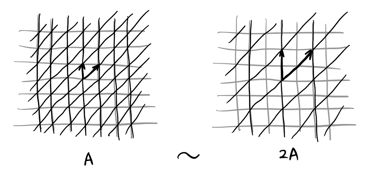
It turns out its converse is also true: All equivalent matrices are scalar multiples of each other! We have:
\((\impliedby)\) is trivial. We only show the direction \((\implies)\) here:
\(\pi(A) = \pi(B)\) implies: \[ \forall v \in V - \{0\}, \pi(Av) = \pi(Bv) \]
By the definition of projective space, \(Av\) and \(Bv\) must be scalar multiple \(\lambda\) of each other and that scalar may depend on \(v\) (We will show that \(\lambda\) is actually independent of \(v\) later): \[ \exists \lambda(v) \in \mathbb{F}^*, Av = \lambda(v)Bv. \tag{7}\]
Pick a basis \(\{e_1, e_2, \cdots, e_n\}\) of \(V\) and take \(v\) to be each of the basis: \[ Ae_i = \lambda(e_i)Be_i, \forall i = 1, 2, \cdots, n. \tag{8}\]
\(\forall v \in V\) is a linear combination of the basis: \(v = \sum \alpha_i e_i\). Multiply \(A\) both sides and from Equation 8, we have: \[ \begin{aligned} Av &= \sum \alpha_i Ae_i = \sum \alpha_i \underbrace{\lambda(e_i) Be_i}_{Ae_i} \\ &= \sum \lambda(e_i) \alpha_i Be_i \end{aligned} \tag{9}\]
But Equation 7 tells us: \[ Av = \lambda(v)Bv = \lambda(v) \sum \alpha_i Be_i. \tag{10}\]
Compare Equation 9 and Equation 10, all \(\lambda\) s must be the same: \[ \lambda(v) = \lambda(e_1) = \lambda(e_2) = \cdots = \lambda(e_n) \equiv \lambda = \text{const}. \]
Therefore, Equation 7 implies: \[ \forall v \in V - \{0\}, Av = \lambda Bv \implies A = \lambda B. \]
We can define the projective linear group \(\text{PGL}(V)\) according to the classification of matrices “up to scalar”:
We know from here that the center of \(\text{GL}(V)\) is exactly \(\mathbb{F}^* I\): \[ \text{ZGL}(V) \equiv Z(\text{GL}(V)) = \mathbb{F}^* I. \]
We know from this post that for any group \(G\), \[ 1 \xrightarrow[]{} Z(G) \hookrightarrow G \twoheadrightarrow \operatorname{Inn}(G) \xrightarrow[]{} 1, \] where \(\text{Inn}(G)\) = \(G/{Z(G)}\). Let \(G = \text{GL}(V)\), then we have: \[ 1 \xrightarrow[]{} \text{ZGL}(V) \hookrightarrow \text{GL}(V) \twoheadrightarrow \operatorname{PGL}(V) \xrightarrow[]{} 1, \] where \[ \text{Inn}(\text{GL}(V)) = \frac{\text{GL}(V)}{\text{ZGL}(V)} = \text{PGL}(V) \]
5.2 Grid of short exact sequence about projective linear groups
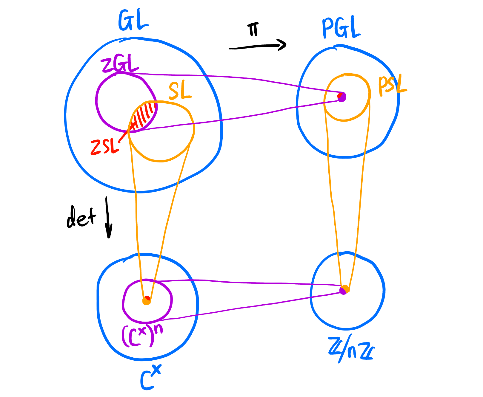
The general linear group \(\text{GL}(V)\), special linear group \(\text{SL}(V)\), their centers \(\text{ZGL}(V)\) and \(\text{ZSL}(V)\), and their projective linear groups \(\text{PGL}(V)\) and \(\text{PSL}(V)\) form the following grid of short exact sequence:
Each row and column in Figure 15 is a short exact sequence8. Everything would be clear if you stare at the cartoon in Figure 16 for a moment.
8 \((\mathbb{C}^{\times})^n\) here means \(\{z^n: z \in \mathbb{C}^{\times }\}\), not \(\mathbb{C}^{\times} \times \cdots \times \mathbb{C}^{\times}\). \(\mathbb{C}^{\times}\) is the same as \(\mathbb{C}^*\), which represents the multiplicative group of non-zero complex numbers.