Solving Laplace’s Equation using Separation of Variables

Learn how to solve stationary heat distribution problem under specific boundary conditions

Takeaway

1 Problem Formulation

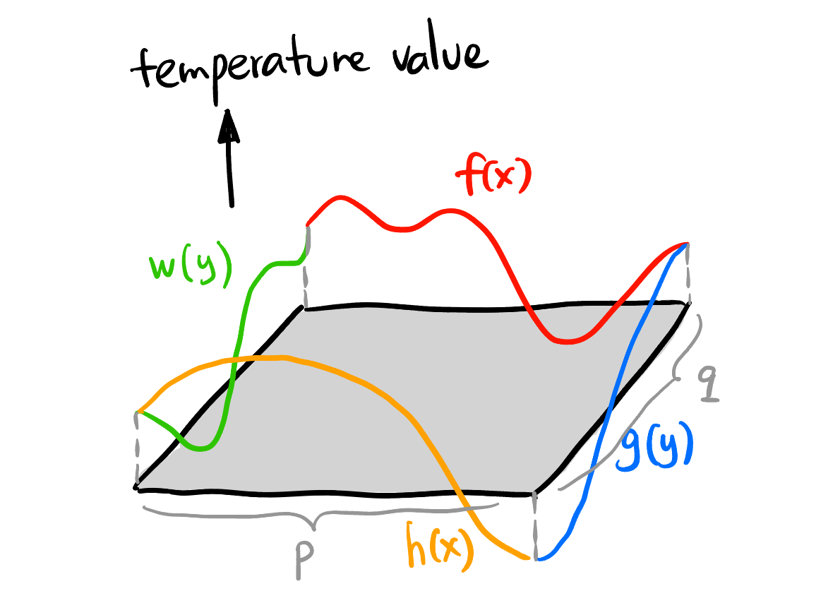
Suppose we have a rectangular sheet of steel sized \(p \times q\). We somehow force the temperature on the boundary of the sheet to be some deterministic function \(f, g, h, w\) shown in Figure 1. When the system settles stablely, what is the temperature distribution \(v(x, y)\) inside the sheet?

Figure 1: How to solve the temperature distribution given boundary condition?

Since the steady heat distribution is governed by the Laplace’s equation. The problem is basically to:

Solve the Laplace’s equation given a (Dirichlet) boundary condition¹ (temperature functions):\[ \nabla^2 v = 0. \]

¹ See here for different types of boundary conditions.

2 Existence and uniqueness of solutions

It’s good habit to always check the existence and uniqueness of a mathematical object.

1. Existence: Does the solution exist?

   In this case, one can guess by life experience that the solution exists since no matter how we force the temperature on the boundary, there must be a temperature distribution inside the sheet.

2. Uniqueness: Does the temperature distribution settles to a unique solution?

   This is not immediately obvious². Could there exist two different stable temperature distributions? The answer is no.

² Not every PDE has a unique solution. For example, the uniqueness of the famous Navier-Stokes equation is still unsolved.

3 Linearity simplifies the problem

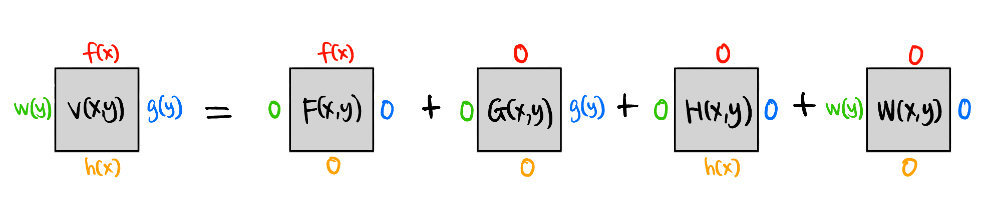
Stare Figure 2 for a while, you will find we just need to solve the steady heat distribution \(F(x, y)\) with an easier boundary condition: \[ \begin{align} F(0, y) &= 0, & y \in [0, q] \tag{BC1} \\ F(0, y) &= 0, & y \in [0, q] \tag{BC2} \\ F(x, 0) &= 0, & x \in [0, p] \tag{BC3} \\ F(x, q) &= f(x), & x \in [0, p] \tag{BC4} \end{align} \tag{1}\]

Figure 2: Linearity of Laplace’s equation simplifies the boundary condition

Simulate the subproblem

4 Separation of variables (SoV)

Suppose \(F(x,y)\) could be written as: \[ F(x,y) = A(x)B(y) \tag{2}\]

Uniqueness legitimize seperation of variables!

Definition 1 Equation 2 is such a bold and unreasonable assumption. Why is that??

It literally doesn’t make any sense, until it indeed gives a solution!

The seperation of variables is just a guess. You will later find that if we continue reasoning using this assumption, we will eventually arrive at a solution that satisfies both the Laplace’s equation and the boundary condition.

Here is the point: The uniqueness theorem guarantees that the solution is unique!, which means the solution we just got is the only solution, though we have no fluent logic to derive it! This is sort of like:

Imagine your primary school teacher ask you to solve the equation: \[ 2x + 3 = 1. \tag{3}\]

You have no idea how to solve it, but you guess that \(x\) satisfies: \[ x + 1 = 0, \] and you get \(x = -1\), which indeed satisfies Equation 3. By Fundamental theorem of algebra, Equation 3 has and only has one solution. Therefore, its solution is \(x = -1\). This is a valid reasoning!!

Then we plugin Equation 2 into the Laplace’s equation: \[ \begin{align*} &\nabla^2 (AB) = 0 \\ \implies\quad &\frac{\partial^2 (AB)}{\partial x^2} + \frac{\partial^2 (AB)}{\partial y^2} = 0 \\ \implies\quad &A_{xx}(x)B(y) + A(x)B_{yy}(y) = 0 \\ \implies\quad &\underbrace{\frac{A_{xx}(x)}{A(x)}}_{\text{function of }x} = \underbrace{-\frac{B_{yy}(y)}{B(y)}}_{\text{function of }y}, \quad \forall (x, y) \in [0, p] \times [0, q]. \end{align*} \]

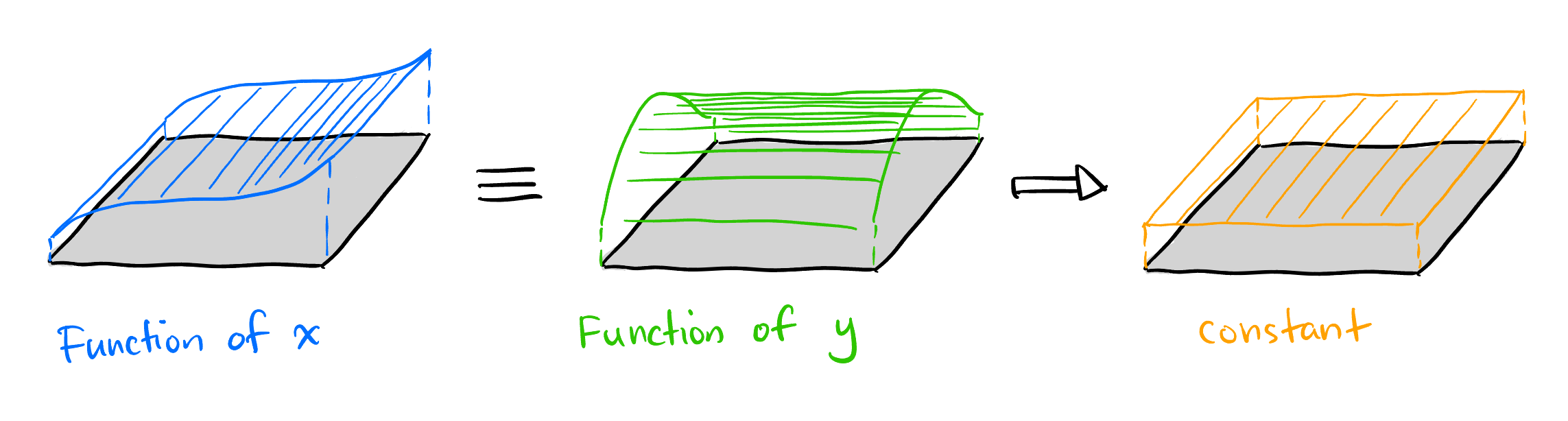
Now here is a very important step, for all point in the rectangle, a function of \(x\) equals a function of \(y\), always. This means they must be constant functions as shown in Figure 3.

\[ \boxed{ \frac{A_{xx}(x)}{A(x)} = -\frac{B_{yy}(y)}{B(y)} = \text{const} \equiv \lambda. } \tag{4}\]

If we denote the constant as \(\lambda\), this is actually problematic because \(\lambda\) could be different numbers as long as \(A_{xx}(x)/A(x)\) and \(-B_{yy}(y)/B(y)\) are equal. We will later see that there are countably \(\lambda\) values that are available and we shall use series to represent the solution.

Figure 3: A function of \(x\) equals a function of \(y\) pointwise forces them constant functions

Now we get two ODEs from Equation 4: \[ \begin{cases} A_{xx} = \lambda A \\ B_{yy} = -\lambda B \end{cases} \tag{5}\]

Refer to Section 7 for the solution of this kind of ODE.

5 Boundary conditions applied

5.1 Determine the sign of \(\lambda\)

Claim

Proposition 1 We claim that: \[ \lambda \le 0. \]

This is because if \(\lambda > 0\), \[ A(x) \in \operatorname{span}_\mathbb{R}\{\cosh(\sqrt{\lambda} x), \sinh(\sqrt{\lambda} x)\}. \] But hyperbolic functions look like the right graph of Figure 5, there is no element in \(\operatorname{span}_\mathbb{R}\{\cosh(\sqrt{\lambda} x), \sinh(\sqrt{\lambda} x)\}\) that equals \(0\) at both ends of the rectangle. Only periodic sinusoidal functions can do that.

From Proposition 1, Equation 5 implies \[ \begin{cases} A(x) \in \operatorname{span}_\mathbb{R}\{\cos(\omega x), \sin(\omega x)\} \cup \{\alpha_1 x + \beta_1\} \\ B(y) \in \operatorname{span}_\mathbb{R}\{\cosh(\omega y), \sinh(\omega y)\} \cup \{\alpha_2 y + \beta_2\} \end{cases} \tag{6}\] where \(-\lambda = \omega^2\)

5.2 Determine valid \(\lambda\) values

5.2.1 Left and right boundary conditions

Let’s start with the easier boundary conditions @BC1 and @BC2.

\(A(x)\) in Equation 6 are just sinusoidal functions or linear functions. If we force it to be zero on the edges, all of a sudden \(\alpha_1\) and \(\beta_1\) should be both zero, and the coefficients before \(\cos(\omega x)\) also must be zero, otherwise the function will never be zero at the line \(x=0\). Also the horizontal length \(p\) must be integer multiple of half period of \(\sin(\omega x)\), i.e., \[ n \cdot \frac{\pi}{\omega} = p, \quad n = 1, 2, 3, \cdots. \]

Therefore, there are only countably many valid \(\omega\), hence countably many valid \(\lambda\): \[ \lambda = -\omega^2 \in \left\{ -\frac{n^2 \pi^2}{p^2} \right\}_{n=1}^\infty. \]

So \(A(x)\) in Equation 6 is in a subspace: \[ \boxed{ A(x) \in \operatorname{span}_\mathbb{R}\left\{\sin\left(\frac{n \pi}{p} x\right)\right\}} \]

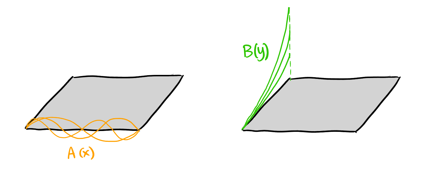
As shown in Figure 4, \(A(x)\) is like the harmonics on a string.

Figure 4: Mental picture for \(A(x)\) and \(B(y)\)

5.2.2 Top and bottom boundary conditions

On top and bottom edges, we have the boundary condition (BC3) and (BC4) in Equation 1.

\(B(y)\) in Equation 6 must obey these boundary conditions. (BC3) in Equation 1 forces \(\beta_2 = 0\), and the coefficients before \(\cosh(\omega y)\) to be zero. So \(B(y)\) in Equation 6 is in a subspace: \[ \boxed{ B(y) \in \operatorname{span}_\mathbb{R}\left\{\sinh\left(\frac{n \pi}{p} y\right)\right\} \cup \{\alpha_2 y\}} \]

5.3 Fourier series for the undetermined coefficients

We have not used the boundary condition (BC4) in Equation 1 yet. Actually, it leads to the introduction to Fourier series! Let’s write what does \(F(x,y)\) looks like up to now: \[ \begin{aligned} F(x, y) &= A(x)B(y) \\ &= c \sin\left(\frac{n \pi}{p} x\right) \sinh\left(\frac{n \pi}{p} y\right) \\ \text{or } &= c' 0 \cdot y \end{aligned} \tag{7}\] where \(c\) depends on the choice of \(n\), \(n\) can be any positive integer. Now we have a very important claim:

Claim

Proposition 2 If we add these valid \(F\) together, the sum is still valid: \[ \boxed{ F(x,y) = \sum_{n=1}^\infty c_n \sin\left(\frac{n \pi}{p} x\right) \sinh\left(\frac{n \pi}{p} y\right).} \tag{8}\]

Think about why!?

Each solution in Equation 7 is a solution to the Laplace’s equation, right? By the superposition principle, their sum is also a solution to the Laplace’s equation!

Here is the most beautiful part: We plugin (BC4) in Equation 1 into Equation 8: \[ F(x, q) = \sum_{n=1}^\infty \underbrace{c_n \sinh\left(\frac{n \pi}{p} q\right)}_{\mathclap{\scriptsize \text{Fourier coefficients of }f(x)}} \sin\left(\frac{n \pi}{p} x\right) = f(x). \tag{9}\]

The \(c_n \sinh(n \pi q/p)\) are just constants, which is exactly the Fourier coefficients of the function \(f(x)\)!

Deriving \(c_n\) through Fourier analysis

We know that a real-valued function \(f(x)\) of period \(T\) could be decomposed as: \[ f(x) = a_0 + \sum_{n=1}^\infty a_n \cos(n \omega_0 x) + \sum_{n=1}^\infty b_n \sin(n \omega_0 x), \tag{10}\] where \[ \begin{cases} a_n &= \frac{2}{T} \langle f, \cos(n \omega_0 x) \rangle \\ b_n &= \frac{2}{T} \langle f, \sin(n \omega_0 x) \rangle \\ a_0 &= \frac{1}{T} \langle f, 1 \rangle. \end{cases} \tag{11}\]

We consider the function \(f(x)\) to be a periodic function with period \(T=2p\) (not \(p\)) since we need \[ \omega_0 = \frac{\pi}{p}. \]

Now we know that all \(a_n = 0\). Compare Equation 11 with Equation 9, \[ b_n = \frac{2}{2p} \left\langle f, \sin\left(\frac{n \pi}{p}x\right) \right\rangle = c_n \sinh\left(\frac{n \pi}{p} q\right). \] Solve for \(c_n\): \[ \begin{aligned} c_n &= \frac{1}{p \sinh\left(\frac{n \pi}{p} q\right)} \left\langle f, \sin\left(\frac{n \pi}{p}x\right) \right\rangle \\ &= \frac{1}{p \sinh\left(\frac{n \pi}{p} q\right)} \int_0^{2p} f(x) \sin\left(\frac{n \pi}{p}x\right) \mathrm{d}x \\ &= \frac{2}{p \sinh\left(\frac{n \pi}{p} q\right)} \int_0^{p} f(x) \sin\left(\frac{n \pi}{p}x\right) \mathrm{d}x. \end{aligned} \]

6 Conclusion

The solution to the simplified boundary condition subproblem is: \[ F(x,y) = \sum_{n=1}^\infty c_n \sin\left(\frac{n \pi}{p} x\right) \sinh\left(\frac{n \pi}{p} y\right), \tag{12}\]

where \(c_n\) satisfies: \[ c_n = \frac{2}{p \sinh\left(\frac{n \pi}{p} q\right)} \int_0^{p} f(x) \sin\left(\frac{n \pi}{p}x\right) \mathrm{d}x. \]

By the superposition principle (shown in Figure 2), the solution to the original problem is the linear combination of the solutions in the form of Equation 12.

7 2nd-order ODE Refresh

7.1 Complex domain solution

Consider the following 2nd-order ODE: \[ \ddot{x} = \lambda x, \tag{13}\] where \(x(t) \in \mathbb{C}, \lambda \in \mathbb{R}\). What function satisfies this special property that if we differentiate it twice, we get itself up to a constant? Exponentials! So we guess: \[ x(t) = e^{rt} \] with \[ r = \pm \sqrt{\lambda}. \]

Therefore, the general solution to Equation 13 is: \[ x(t) = c_1 e^{\sqrt{\lambda} t} + c_2 e^{-\sqrt{\lambda} t}, \tag{14}\] where \(c_1, c_2 \in \mathbb{C}\) are constants. Done!

We can use different notation according to the sign of \(\lambda\):

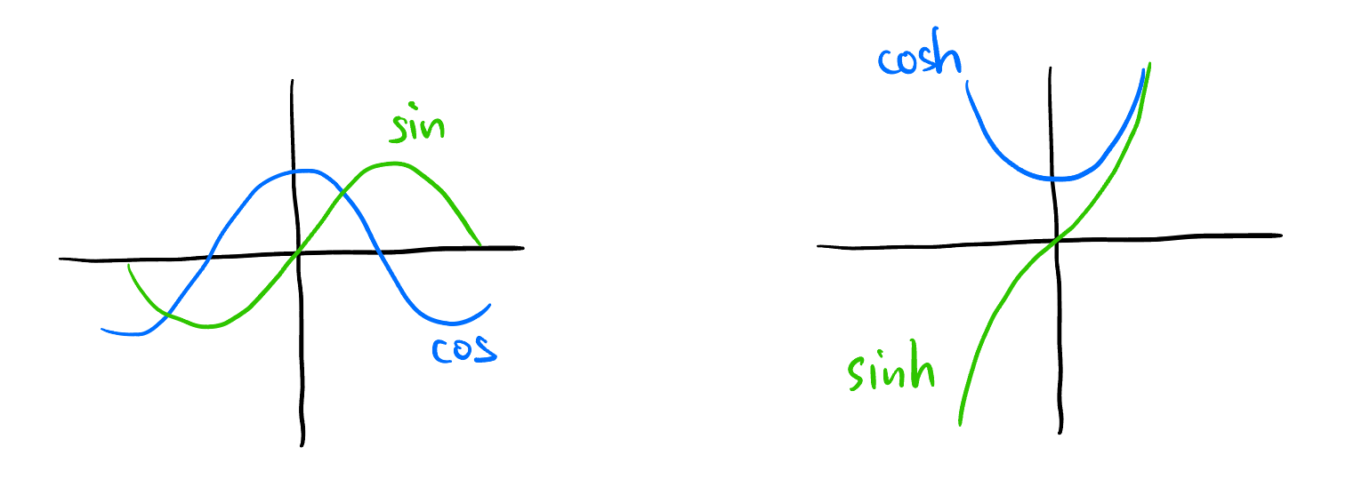
1. \(\lambda < 0\): Let \(-\lambda = \omega^2\), then Equation 14 can also be written as: \[ x(t) = c_1' \cos(\omega t) + c_2' \sin(\omega t) \quad (c_1', c_2' \in \mathbb{C}) \tag{15}\] since \[ \operatorname{span}_\mathbb{C}\{e^{i\omega t}, e^{-i\omega t}\} = \operatorname{span}_\mathbb{C}\{\cos(\omega t), \sin(\omega t)\} \]

2. \(\lambda > 0\): Let \(\lambda = a^2\), then Equation 14 can also be written as: \[ x(t) = c_1'' \cosh(at) + c_2'' \sinh(at) \quad (c_1'', c_2'' \in \mathbb{C}) \tag{16}\] since \[ \operatorname{span}_\mathbb{C}\{e^{at}, e^{-at}\} = \operatorname{span}_\mathbb{C}\{\cosh(at), \sinh(at)\}. \]

3. \(\lambda = 0\):

\[ \begin{align*} &\ddot{x} = 0 \\ \implies\quad &\dot{x} = \alpha \\ \implies\quad &x(t) = \alpha x + \beta \end{align*} \]

Figure 5: The graph of trigonometric and hyperbolic functions

7.2 Real domain solution

The solution of Equation 13 when \(x(t)\) is confined to \(\mathbb{R}\) is very simple. One just need to confine \(c_1', c_2'\) in Equation 15 and \(c_1'', c_2''\) in Equation 16 to \(\mathbb{R}\): \[ x(t) = c_1 \cos(\omega t) + c_2 \sin(\omega t) \quad (\lambda < 0, -\lambda = \omega^2, c_1, c_2 \in \mathbb{R}) \] and \[ x(t) = c_1 \cosh(at) + c_2 \sinh(at) \quad (\lambda > 0, \lambda = a^2, c_1, c_2 \in \mathbb{R}). \]